Rationale for RonDB

The idea to build NDB Cluster that later was merged into the MySQL framework and became RonDB came from the analysis Mikael Ronström did as part of his Ph.D studies. He worked at Ericsson and participated in a study about the new UMTS mobile system developed in Europe that later turned into 3G. As part of this study, there was a lot of work on understanding the requirements of network databases for the UMTS system. In addition, he studied several related areas like Number Portability, Universal Personal Telephony, Routing Servers, Name Servers (e.g. DNS Servers), Intelligent Network Servers. Other application areas he studied were News-on-demand, multimedia email services, event data services and finally, he studied data requirements for genealogy.

Areas of study were requirements on response times, transaction rates and availability and a few more aspects.

These studies led to a few conclusions:

1. Predictable response time requirements required a main memory database

2. Predictable response time requirements required using a real-time scheduler

3. Throughput requirements required a main memory database

4. Throughput requirements required building a scalable database

5. Availability requirements required using replicated data

6. Availability requirements required using a Shared-Nothing Architecture

7. Availability requirements means that applications should not execute inside the DBMS unless in a protected manner

8. Certain applications need to store large objects on disk inside the DBMS

9. The most common operation is key lookup

10. Most applications studied were write-intensive

Separation of Data Server and Query Server

In MySQL, there is a separation of the Query Server and the Data Server functionality. The Query Server is what takes care of handling the SQL queries and maps those to lower layers call into the Data Server. The API to the Data Server in MySQL is the storage engine API.

Almost all DBMS have a similar separation between Data Server and Query Server. However, there are many differences in how to locate the interfaces between Data Server and Query Server and Query Server and the application.

Fully integrated model

The figure below shows a fully integrated model where the application is running in the same binary as the DBMS. This gives very low latency. The first database product Mikael Ronström worked on was called DBS and was a database subsystem in AXE that generated PLEX code (PLEX was the programming language used in AXE) from SQL statements. This is probably the most efficient SQL queries that exists, a select query that read one column using a primary key took 2 assembler instructions in the AXE CPU (APZ).

There were methods to query and update the data through external interfaces, but those were a lot slower compared to internal access.

This model is not flexible, it’s great in some applications, but the applications have to be developed with the same care as the DBMS since it is running in the same memory. It is not a model that works well to get the best availability. It doesn’t provide the benefits of scaling the DBMS in many different directions.

The main reason for avoiding this approach is the high availability requirement. If the application gets a wrong pointer and writes some data out of place, it can change the data inside the DBMS. Another problem with this approach is that it becomes difficult to manage in a shared-nothing architecture since the application will have to be colocated with its data for the benefits to be of any value.

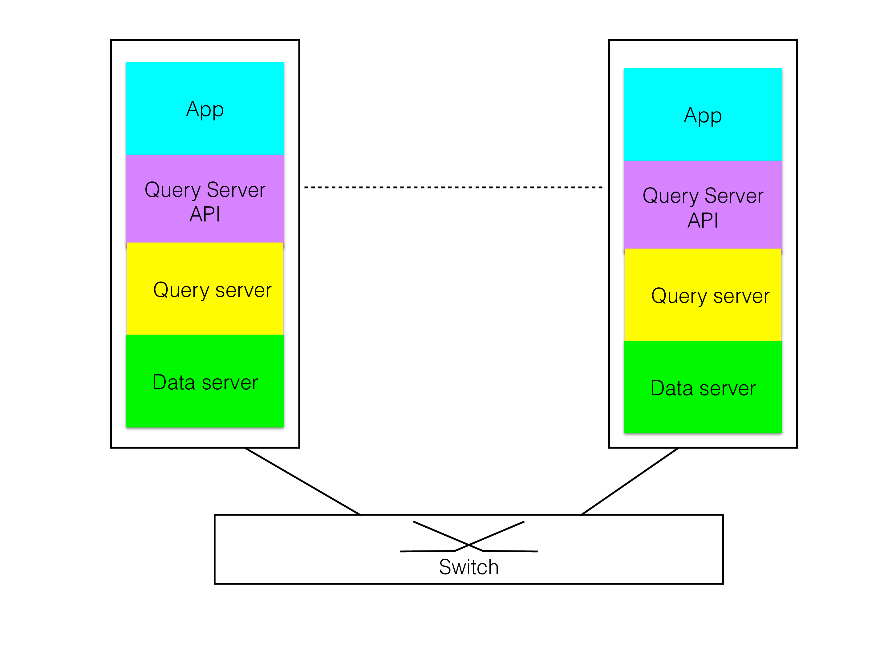
Colocated Query Server and Data Server

The next step that one would take is to separate the Query Server from the API, but still colocating the Query Server and the Data Server as shown in the figure.

This is the model used by most DBMSs. This makes the DBMS highly specialized, if the external API is using SQL, every access to the Data Server has to go through SQL. If the external API is LDAP, every access has to go through LDAP.

Some examples of this model are Oracle, IBM DB2, MySQL/InnoDB and various LDAP server solutions. Its drawback is that it isn’t good to handle mixed workloads that use both complex queries where a language like SQL is suitable and many simple queries that are the bulk of the application.

The Query Server functionality requires a lot of code to manage all sorts of complex queries, it requires a flexible memory model that can handle many concurrent memory allocations from many different threads.

The Data Server is much more specialized software, it has a few rather simple queries that it can handle, the code to handle those are much smaller compared to the Query Server functionality.

Thus even in this model, the argument for separating the Query Server and the Data Server due to availability requirements is a strong argument. Separating them means that there is no risk for flaws in the Query Server code to cause corruption of the data. The high availability requirements of NDB led to a choice of model where we wanted to minimize the amount of code that had direct access to the data.

Most DBMSs use SQL or some other high-level language to access it. The translation from SQL to low-level primitives gives a fairly high overhead. The requirements on high throughput of primary key operations for NDB meant that it was important to provide an access path to data which didn’t require the access to go through a layer like SQL.

These two arguments were strong advocates for the separation of the query server and Data Server functionality.

Thus RonDB although designed in the 1990s was designed as a key-value database with SQL capabilities as an added value.

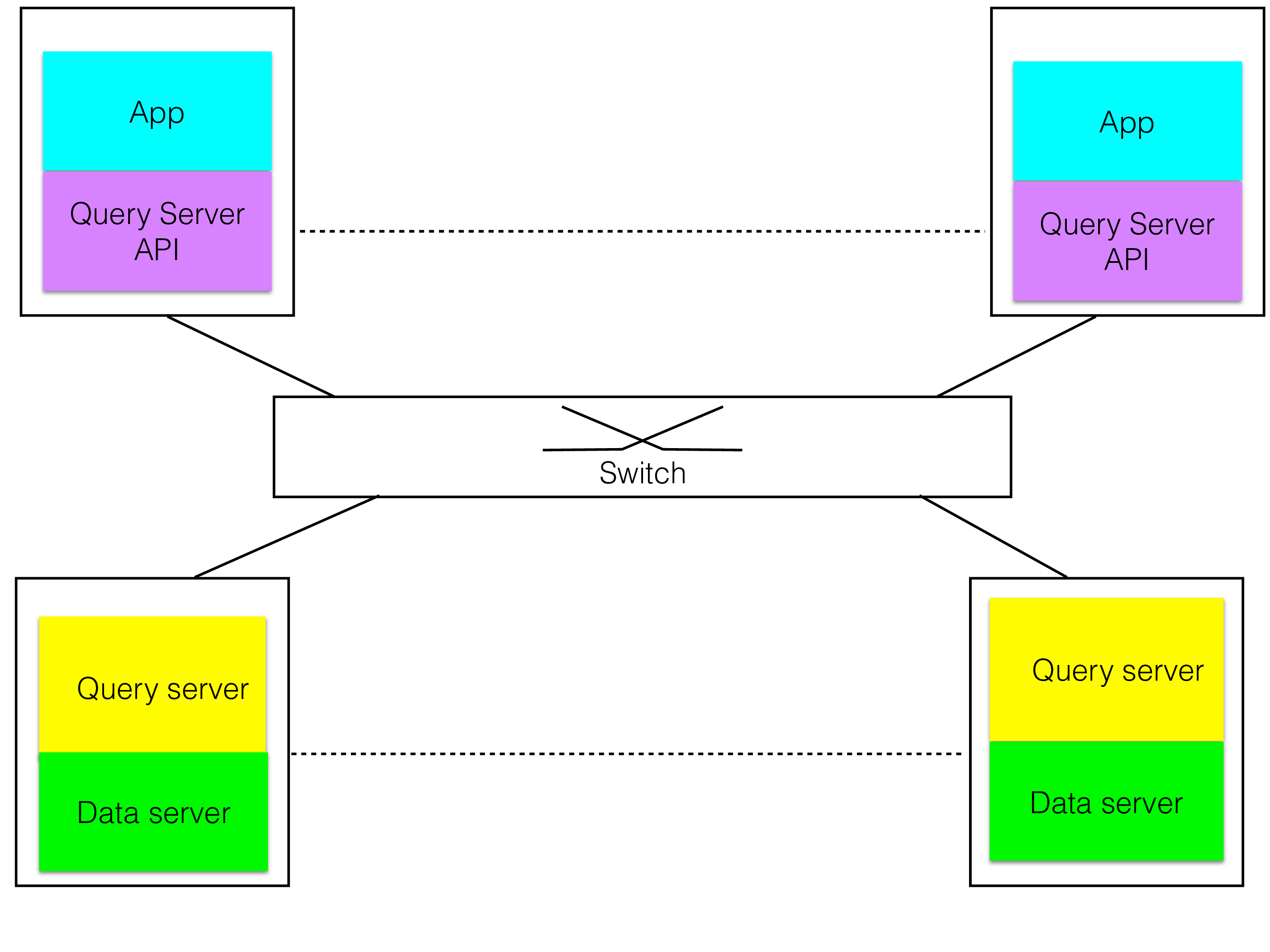
RonDB Model

The above reasoning led to the conclusion to separate the Query Server facilities from the Data Server facility. The Data Server provides a low-level API where it is possible to access rows directly through a primary key or unique key and it is possible to scan a table using a full table scan or an index scan on an ordered index. It is possible to create and alter metadata objects. It is possible to create asynchronous event streams that provide information about any changes to the data in the Data Server. The Data Server will handle the recovery of data, it will handle the data consistency and replication of data.

This ensures that the development of the Data Server can be focused and there is very little interaction with the development of the Query Server parts. It does not have to handle SQL, LDAP, query optimization, file system APIs or any other higher-level functionality required to support the Query Server functionality. This greatly diminishes the complexity of the Data Server.

Later on, we added capabilities to perform a bit more complex query executions to handle complex join operations.

Benefits of RonDB Model

The figure of the RonDB model above shows how a network API between the Data Server and the Query Server it is possible to both use it with SQL as the API, to access the Data Server API directly and to use the LDAP API to the same Data Servers that supports SQL and applications using the Data Server API directly and file system services on top of RonDB. Thus providing a flexible application development.

The nice thing with the development of computers is that they develop to get more and more bandwidth for networking. In addition, it is possible to colocate the Query Server process and the Data Server process on the same machine. In this context, the integration of the Query Server and the Data Server is almost at the same level as the integration when they are part of the same process. Some DBMSs use the colocated model but still use multiple processes to implement the DBMS.

This separation of the Data Server and the Query Server has been essential for RonDB. It means that one can use RonDB to build an SQL server, it means that you can use RonDB to build an LDAP server, you can use it to build various networking servers, metadata servers for scalable file systems and it means that you can use RonDB to build a file server and you can even use it to build a distributed block device to handle petabytes of data. We will discuss all those use cases and a few more later on in this book.

Drawbacks of RonDB Model

There is a drawback to the separation of the Query Server and the Data Server. To query the data we have to pass through several threads to access the data. This increases the latency of accessing the data when you use SQL access. Writing a combined Query Server and Data Server to implement an SQL engine is always faster for a single DBMS server. RonDB is however designed for a distributed environment with replication and sharding from the ground up.

We have worked hard to optimize SQL access in the single server case, and we’re continuing this work. The performance is now almost at par with the performance one can achieve with a combined Query Server and Data Server.

Understanding the RonDB Model

An important part of the research work was to understand the impact of the separation of the Data Server and the Query Server.

Choosing a network-based protocol as the Data Server API was a choice to ensure the highest level of reliability of the DBMS and its applications. We have a clear place where we can check the correctness of the API calls and only through this API can the application change the data in the Data Server.

Another reason that made it natural to choose a network protocol as API was that the development of technologies for low-latency and high bandwidth had started already in the 1990s. The first versions of NDB Cluster had an SCI transporter as its main transporter which ensured that communication between computers could happen in microseconds. TCP/IP sockets have since replaced it since SCI and Infiniband now have support for TCP/IP sockets that is more or less as fast as direct use of SCI and Infiniband.

One more reason for using a network protocol as API is that it enables us to build scalable Data Servers.

As part of the research, we looked deeply into the next-generation mobile networks and their use of network databases. From these studies, it was obvious that the traffic part of the applications almost always made simple queries, mostly key lookups and in some cases slightly more complex queries were used. Thus the requirements pointed clearly at developing RonDB as a key-value database.

At the same time, there are management applications in the telecom network, these applications will often use more complex queries and will almost always use some sort of standard access method such as SQL.

Normally the traffic queries have strict requirements on response times whereas the management applications have less strict requirements on response times.

It was clear that there was a need for both a fast path to the data as well as standard APIs used for more complex queries and for data provisioning.

From this, it was clear that it was desirable to have a clearly defined Data Server API in a telecom DBMS to handle most of the traffic queries. Thus we can develop the Data Server to handle real-time applications while at the same time supporting applications that focus more on complex queries and analyzing the data. Applications requiring real-time access can use the same cluster as applications with less requirements on real-time access but with needs to analyze the data.

How we did it

To make it easier to program applications we developed the C++ NDB API that is used to access the RonDB Data Server protocol.

The marriage between MySQL and NDB Cluster was a natural one since NDB Cluster had mainly focused on the Data Server parts and by connecting to the MySQL Server we had a natural implementation of the Query Server functionality. Based on this marriage we have now created RonDB as a key-value database optimized for the public cloud.

The requirements for fast failover times in telecom DBMSs made it necessary to implement RonDB as a shared-nothing DBMS.

The Data Server API has support for storing relational tables in a shared-nothing architecture. The methods available in the RonDB Data Server API are methods for key-value access for read and write, scan access using full table scan and ordered index scans. In 7.2 we added some functionality to pushdown join execution into the Data Server API. There is a set of interfaces to create tables, drop tables, create foreign keys, drop foreign keys, alter a table, adding and dropping columns, adding and dropping indexes and so forth. There is also an event API to track data changes in RonDB.

To decrease the amount of interaction we added an interpreter to the RonDB Data Server, this can be used for simple pushdown of filters, it can be used to perform simple update operations (such as increment a value) and it can handle LIKE filters.

Advantages and Disadvantages

What are the benefits and disadvantages of these architectural choices been over the 15 years NDB has been in production usage?

One advantage is that RonDB can be used for many different things.

One important use case is what it was designed for. There are many good examples of applications written against any of the direct NDB APIs to serve telecom applications, financial applications and web applications while still being able to access the same data through an SQL interface in the MySQL Server. These applications use the performance advantage that makes it possible to scale applications to as much as hundreds of millions of operations per second.

Another category in popular use with NDB is to implement an LDAP server as a Query Server on top of the NDB Data Server (usually based on OpenLDAP). This would have been difficult using a Query Server API since the Query Server adds a significant overhead to simple requests.

The latest example of use cases is to use the Data Server to implement a scalable file system. This has been implemented by HopsFS in replacing the Name Server in Hadoop HDFS with a set of Name Servers that use a set of NDB Data Servers to store the actual metadata. Most people who hear about such an architecture being built on something with MySQL in the name will immediately think of the overhead in using an SQL interface to implement a file system. But it isn’t the SQL interface that is used, it is implemented directly on top of the Java implementation of the NDB API, ClusterJ.

The final category is using RonDB with the SQL interface. Many applications want RonDB’s high availability but still want to use an SQL interface. Many pure SQL applications see the benefit of the data consistency of MySQL Servers using RonDB and the availability and scalability of RonDB.

The disadvantage is that DBMSs that have a more direct API between the Query Server and the Data Server will get benefits in that they don’t have to go over a network API to access its data. With RonDB you pay this extra cost to get higher availability, more flexible access to your data and higher scalability and more predictable response times.

This cost was a surprise to many early users of NDB. We have worked hard since the inception of NDB Cluster into MySQL to ensure that the performance of SQL queries is as close as possible to the colocated Query Server and Data Server APIs. We’ve gotten close and we are continuously working on getting closer. Early versions lacked many optimizations using batching and many other important optimizations have been added over the years.

The performance of RonDB is today close to the performance of MySQL/InnoDB for SQL applications and as soon as some of the parallelization abilities of RonDB are made use of, the performance is better.

By separating the Data Server and the Query Server we have made it possible to work on parallelizing some queries in an easy manner. This makes the gap much smaller and for many complex queries RonDB will outperform local storage engines.

Predictable response time requirements

As part of Mikael Ronström’s Ph.D thesis, databases in general was studied and looked at what issues DBMSs had when executing in an OS. What was discovered was that the DBMS is spending most of its time in handling context switches, waiting for disks and in various networking operations. Thus a solution was required that avoided the overhead of context switches between different tasks in the DBMS while at the same time integrating networking close to the operations of the DBMS.

When analyzing the requirements for predictable response times in NDB Cluster based on its usage in telecom databases two things were important. The first requirement is that we need to be able to respond to queries within a few milliseconds (today down to tens of microseconds). The second requirement is that we need to do this while at the same time supporting a mix of simple traffic queries combined with several more complex queries.

The first requirement was the main requirement that led to NDB Cluster using a main memory storage model with durability on disk using a REDO log and various checkpoints.

The second requirement is a bit harder to handle. To solve the second requirement in a large environment with many CPUs can be done by allowing the traffic queries and management queries to run on different CPUs. This model will not work at all in a confined environment with only 1-2 CPUs and it will be hard to get it to work in a large environment since the usage of the management queries will come and go quickly.

The next potential solution is to simply leave the problem to the OS. Modern OSs of today use a time-sharing model. However, each time quanta is fairly long compared to our requirement of responding within parts of a millisecond.

Another solution would be to use a real-time operating system, but this would make the product too limited. Even in the telecom application space real-time operating systems are mostly used in the access network.

There could be simple transactions with only a single key lookup. Number translation isn’t much more than this simple key lookup query. At the same time, most realistic transactions look similar to the one below where a transaction comprises several lookups, index scans and updates.

There are complex queries that analyze data (these are mostly read-only transactions) and these could do thousands or more of these lookups and scans and they could all execute as part of one single query. It would be hard to handle the predictability of response times if these were mixed using normal threads using time-sharing in the OS.

Most DBMS today use the OS to handle the requirements on response times. As an example, if one uses MySQL/InnoDB and send various queries to the MySQL Server, some traffic queries and some management queries, MySQL will use different threads for each query. MySQL will deliver good throughput in the context of varying workloads since the OS will use time-sharing to fairly split the CPU usage amongst the various threads. It will not be able to handle the response time requirements of parts of a millisecond with a mixed load of simple and complex queries.

Most vendors of key-value databases have now understood that the threading model isn’t working for key-value databases. However, RonDB has an architecture that has slowly improved over the years and is still delivering the best latency and throughput of the key-value databases available.

AXE VM

When designing NDB Cluster we wanted to avoid this problem. NDB was initially designed within Ericsson. In Ericsson, a real-time telecom switch had been developed in the 70s, the AXE. The AXE is still in popular use today and new versions of it are still developed. AXE had a solution to this problem which was built around a message passing machine.

AXE had its own operating system and at the time its own CPUs. The computer architecture of an AXE was very efficient and the reason behind this was exactly that the cost of switching between threads was almost zero. It got this by using asynchronous programming using modules called blocks and messages called signals.

Mikael Ronström spent a good deal of the 90s developing a virtual machine for AXE called AXE VM that inspired the development of a real product called APZ VM (APZ is the name of the CPU subsystem in the AXE). This virtual machine was able to execute on any computer.

The AXE VM used a model where execution was handled as execution of signals. A signal is simply a message, this message contains an address label, it contains a signal number and it contains data of various sizes. A signal is executed inside a block, which is a self-contained module that owns all its data. The only manner to get to the data in the block is by sending a signal to the block.

The AXE VM implemented a real-time operating system inside a normal operating system such as Windows, Linux, Solaris or Mac OS X. This solves the problem with predictable response time, it gives low overhead for context switching between execution of different queries and it makes it possible to integrate networking close to the execution of signals.

The implementation of RonDB borrows ideas from the AXE architecture and implements an architecture with several blocks and signals sent between those blocks. A nice side effect of this is that the code is using a message passing oriented implementation. This is nice when implementing a distributed database engine.

The first figure shows how RonDB uses blocks with its own data and signals passed between blocks to handle things. This was the initial architecture.

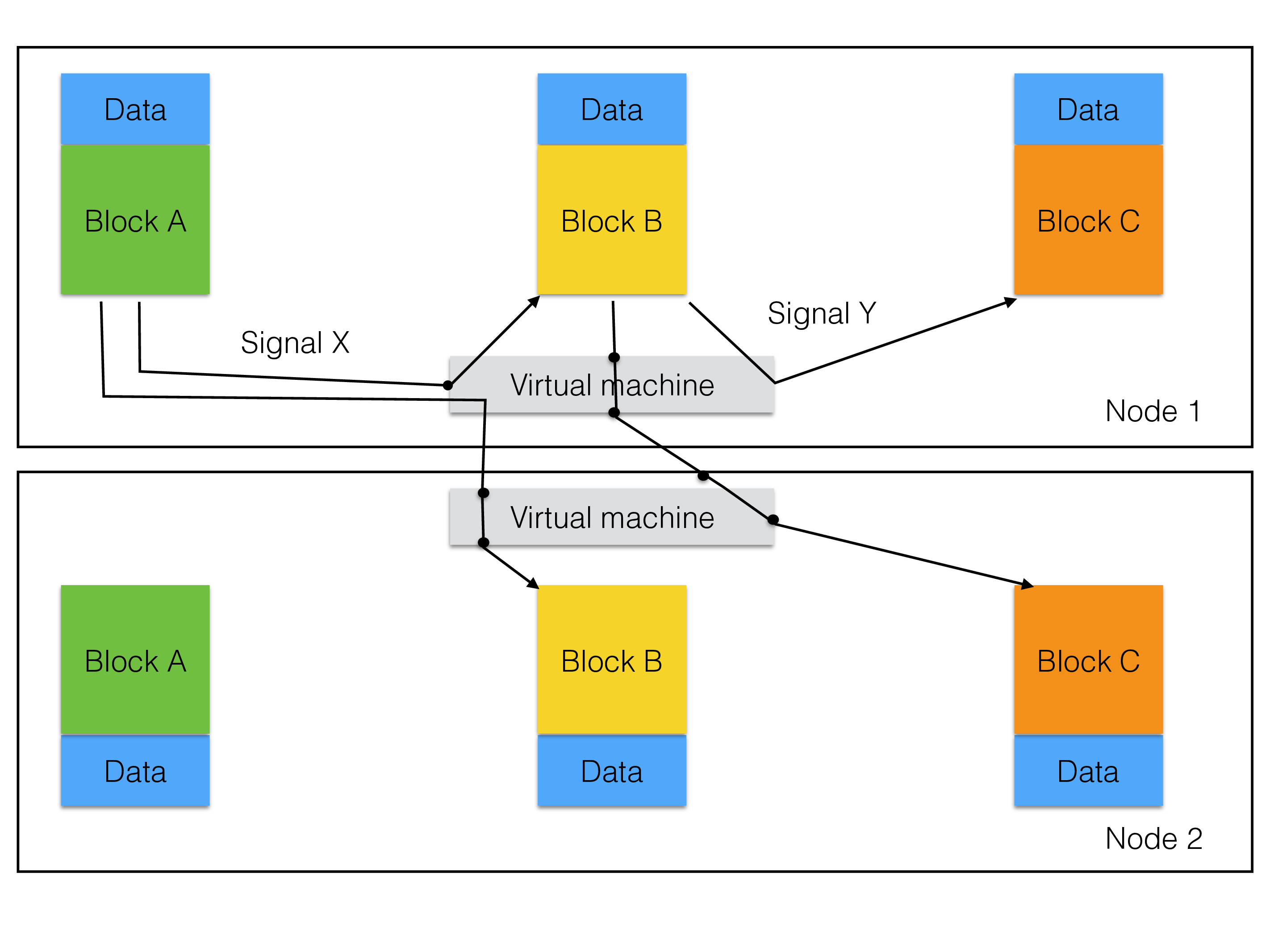
The figure below shows how the full RonDB architecture looks like in the data nodes. It shows how it uses the AXE architecture to implement a distributed message passing system using blocks and a VM (virtual machine) that implements message passing between blocks in the same thread, message passing between blocks in the same process and message passing between blocks in different processes, it can handle different transporters of the messages between processes (currently only TCP/IP sockets), scheduling of signal execution and interfacing the OS with CPU locking, thread priorities and various other things.

We have further advanced this such that the performance of a data node is now much higher and can nicely fill up a 16-core machine and a 32-core machine and with some drop of scalability even a 48-core machine. The second figure shows the full model used in RonDB.

A signal can be local to the thread in which case the virtual machine will discover this and put it into the scheduler queue of the own thread. It could be a message to another block in the same node but in a different thread. In this case we have highly optimized non-locking code to transfer the message using memory barriers to the other thread and place it into the scheduler queue of this thread. A message could be targeted for another node, in this case we use the send mechanism to send it over the network using a TCP/IP socket.

The target node could be another data node, it could be a management server or a MySQL Server. The management server and MySQL Server uses a different model where each thread is its own block. The addressing label contains a block number and a thread ID, but this label is interpreted by the receiver, only the node ID is used at the send side to determine where to send the message. In the data node a receiver thread will receive the message and will transport it to the correct block using the same mechanism used for messages to other threads.

Another positive side effect of basing the architecture on the AXE was that we inherited an easy model for tracing crashes. Signals go through so-called job buffers. Thus we have access to a few thousand of the last executed signals in each thread and the data of the signals. This trace comes for free. In addition, we borrowed another concept called Jump Address Memory (JAM), this shows the last jumps that the thread did just before the crash. This is implemented through a set of macros that we use in a great number of places in the code. This has some overhead, but the payback is huge in terms of fixing crashes. It means that we can get informative crash traces from the users that consume much less disk space than a core file would consume and still it delivers more real information than the core files would do. The overhead of generating those jump addresses is on the order of 10-20% in the data node threads. This overhead has paid off in making it a lot easier to support the product.

The AXE VM had a lot of handling of the language used in AXE called PLEX. This is no longer present in RonDB. But RonDB still is implemented using signals and blocks. The blocks are implemented in C++ and in AXE VM it was possible to have such blocks, they were called simulated blocks. In NDB all blocks are nowadays simulated blocks.

How does it work

How does this model enable response times of down to parts of a millisecond in a highly loaded system?

First of all it is important to state that RonDB handles this.

There are demanding users in the telecom, networking and in financial sectors and lately in the storage world that expects to run complex transactions involving tens of different key lookups and scan queries and that expects these transactions to complete within a few milliseconds at 90-95% load in the system.

For example in the financial sector missing the deadline might mean that you miss the opportunity to buy or sell some stock equity in real-time trading. In the telecom sector your telephone call setup and other telco services depends on immediate responses to complex transactions.

At the same time, these systems need to ensure that they can analyze the data in real-time, these queries have less demanding response time requirements, running those queries isn’t allowed to impact the response time of the traffic queries.

The virtual machine model implements this by using a design technique where each signal is only allowed to execute for a few microseconds. A typical key lookup query in modern CPUs takes less than two microseconds to execute. Scanning a table is divided up into scanning a few rows at a time where each such scan takes less than ten microseconds. All other maintenance work to handle restarts, node failures, aborts, creating new tables and so forth is similarly implemented with the same requirements on signal execution.

Thus a typical traffic transaction is normally handled by one key lookup or a short scan query and the response is sent back to the API node. A transaction consists of several such interactions normally in the order of tens of such queries. Thus each interaction needs to complete within 100-200 microseconds to handle response times of a few milliseconds.

RonDB can handle this response time requirement even when 20-30 messages are queued up before the message given that each message will only take on the order of 1-2 microseconds to execute. Thus most of the time is still spent in the transporter layer sending the message and receiving the message.

A complex query will execute in this model by being split into many small signal executions. Each time a signal is completed it will put itself back into the queue of signals and wait for its next turn.

Traffic queries will always have the ability to meet strict requirements on response time. Another nice thing about this model is that it will adapt to varying workloads within a few microseconds. If there is currently no traffic queries to execute, the complex query will get the CPU to itself since the next signal will execute immediately after being put on the queue.

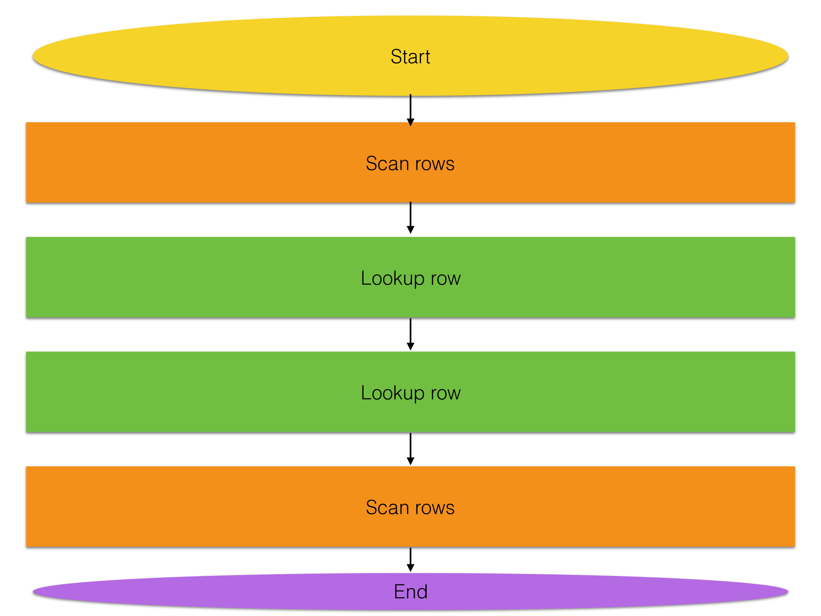
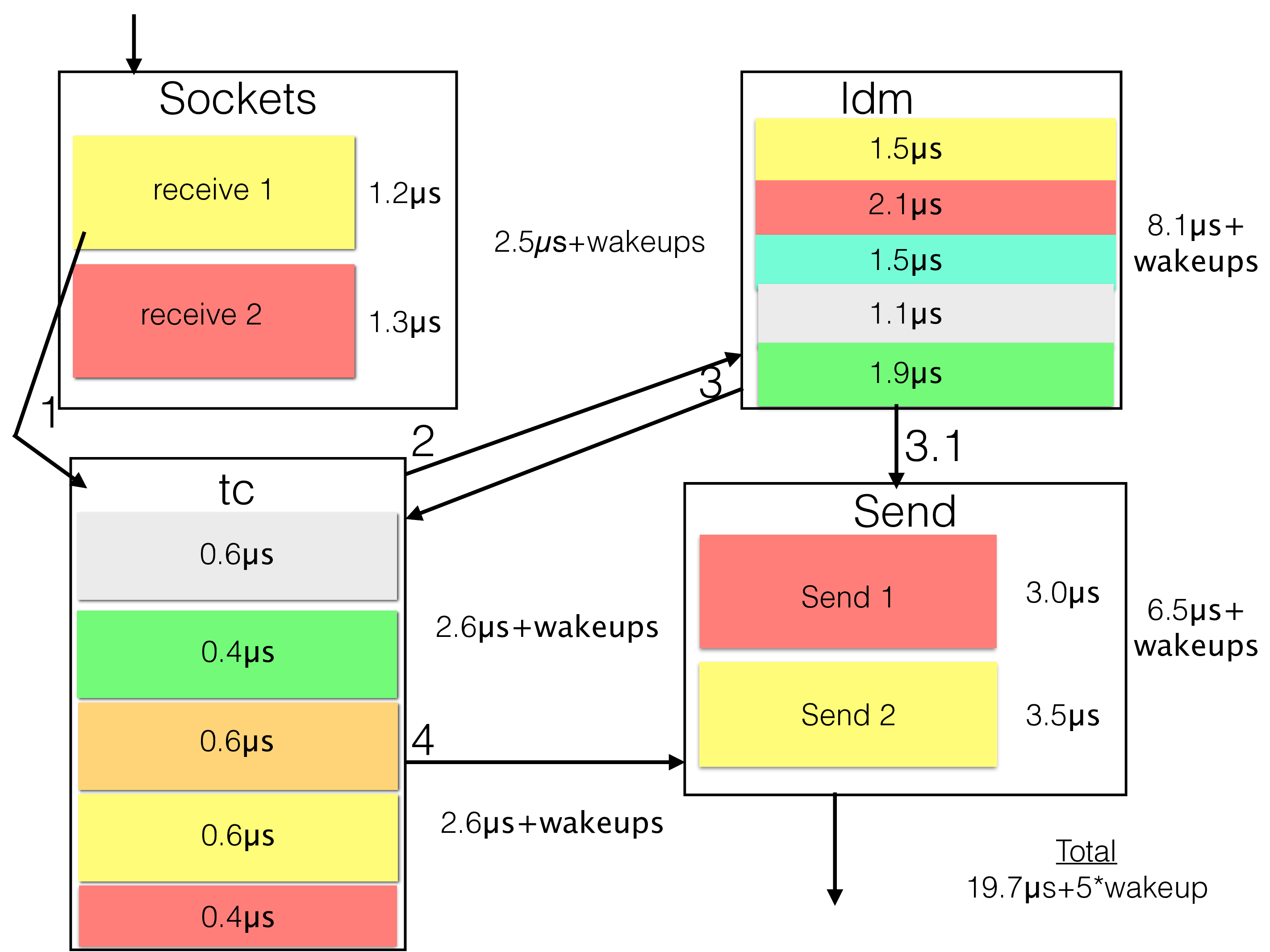
In the figure below we have shown an example of how the execution of a primary key read operation might be affected by delays in the various steps it handles as part of the lookup. In this example case (the execution times are rough estimates of an example installation) the total latency to execute the primary key lookup query is 19.7 microseconds plus the time for a few thread wakeups. The example case represents a case where load is around 80%. We will go through in detail later in this book what happens during the execution of a transaction.

The figure clearly shows the benefits of avoiding wakeups. Most of the threads in the RonDB data nodes can spin before going back to sleep. By spinning for a few hundred microseconds in the data nodes the latency of requests will go down since most of the wakeup times disappear. Decreasing the wakeup times also benefits query execution time positively since the CPU caches are warmer when we come back to continue executing a transaction.

In a benchmark we often see that performance scales better than linearly going from one to four threads. The reason is that with a few more active transactions the chance of finding threads already awake increases and thus the latency incurred by wakeups decreases as load increases.

We opted for a functional division of the threads. We could have put all parts into one thread type that handles everything. This would decrease the amount of wakeups needed to execute one lookup. It would decrease the scalability at the same time. This is why RonDB implements an adaptive CPU spinning model that decreases the amount of wakeup latency.

There is one more important aspect of this model. As the load increases, two things happen. First, we execute increasingly more signals every time we have received a set of signals. This means that the overhead to collect each signal decreases. Second, executing larger and larger sets of signals means that we send larger and larger packets. Thus the cost per packet decreases. Thus RonDB data nodes execute more and more efficiently as load increases. This is an important characteristic that avoids many overload problems.

This means in the above example that as load increases the amount of wakeups decrease, we spend more time in queues, but at the same time we spend less time in waiting for wakeups. Thus the response time is kept almost stable until we reach a high load. The latency of requests starts to dramatically increase around 90-95% load. Up until 90% load the latency is stable and you can get very stable response times.

The functional division of threads makes RonDB data nodes behave better compared to if everything was implemented as one single thread type. If the extra latency for wakeups one can use the spinning feature discussed above. This has the effect that we can get very low response times in the case of a lightly loaded cluster. Thus we could get response times down to below 30 microseconds for most operation types. Updating transactions will take a bit longer since they have to visit each node several times before the transaction is complete, a minimum of 5 times for a simple update transaction and a minimum of 7 times for a simple update transaction on a table that uses the read backup feature (explained in a later chapter).

The separation of Data Server and Query Server functionality makes it possible to use different Query Server for traffic queries to the ones used for complex queries. In the RonDB model, this means that you can use a set of MySQL Servers in the cluster to handle short real-time queries. You can use a different set of MySQL Servers to handle complex queries. Thus RonDB can handle real-time requirements in a proper configuration of the cluster when executing SQL queries.

The separation of Data Server and Query Server functionality might mean that RonDB has a slightly longer minimum response time compared to a local storage engine in MySQL, but RonDB will continue to deliver low and predictable response times using varying workloads and executing at high loads.

One experiment that was done when developing pushdown join functionality showed that the latency of pushed down joins was the same when executing in an idle cluster compared to a cluster that performed 50.000 update queries per second concurrently with the join queries.

We have now built a benchmark structure that makes it very easy to combine running an OLTP benchmark combined with an OLAP benchmark running at the same time in RonDB.

RonDB and multi-core architectures

In 2008 the MySQL team started working hard on solving the challenge that modern processors have more CPUs and CPU cores. Before that the normal server computer had 2 CPUs and sometimes even 4 CPUs. MySQL scaled well to those types of computers. However, when the single-threaded performance was harder and harder to further develop the processor manufacturers started developing processors with a lot more CPUs and CPU cores. Lately, we’ve seen the introduction of various server processors from AMD, Intel and Oracle that have 32 CPU cores per processor and each CPU core can have 2-8 CPUs depending on the CPU architecture (2 for x86 and 8 for SPARC and Power).

MySQL has now developed such that each MySQL Server can scale beyond 64 CPUs and each RonDB data node can scale to around 64 CPUs as well. Modern standard dual socket servers come equipped with up to 128 CPUs for x86s and up to 512 CPUs for SPARC computers.

The development of more and more CPUs per generation has slowed down now compared to a few years ago. But both MySQL Server and RonDB data nodes are developed in such a fashion that we try to keep up with the further development of scalability in modern computers.

Both NDB data nodes and MySQL Server nodes can scale to at least a large processor with 32 CPU cores for x86. The RonDB architecture still makes it possible to have more than one node per computer. Thus the RonDB architecture will work nicely for all types of computers, even with the largest computers. NDB is tested with computers that have up to 120 CPUs for x86 and up to 1024 CPUs with SPARC machines.

Shared-nothing architecture

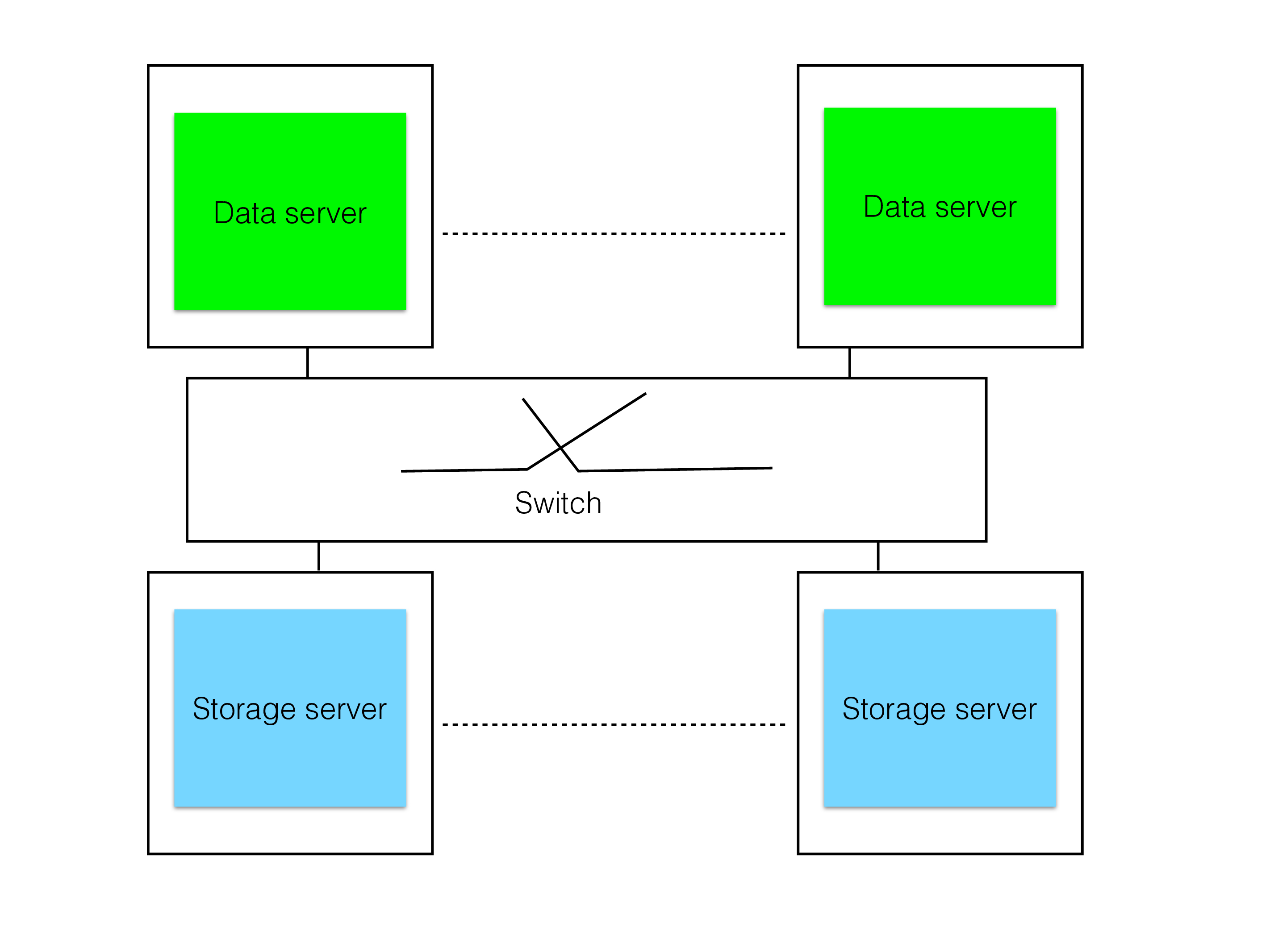
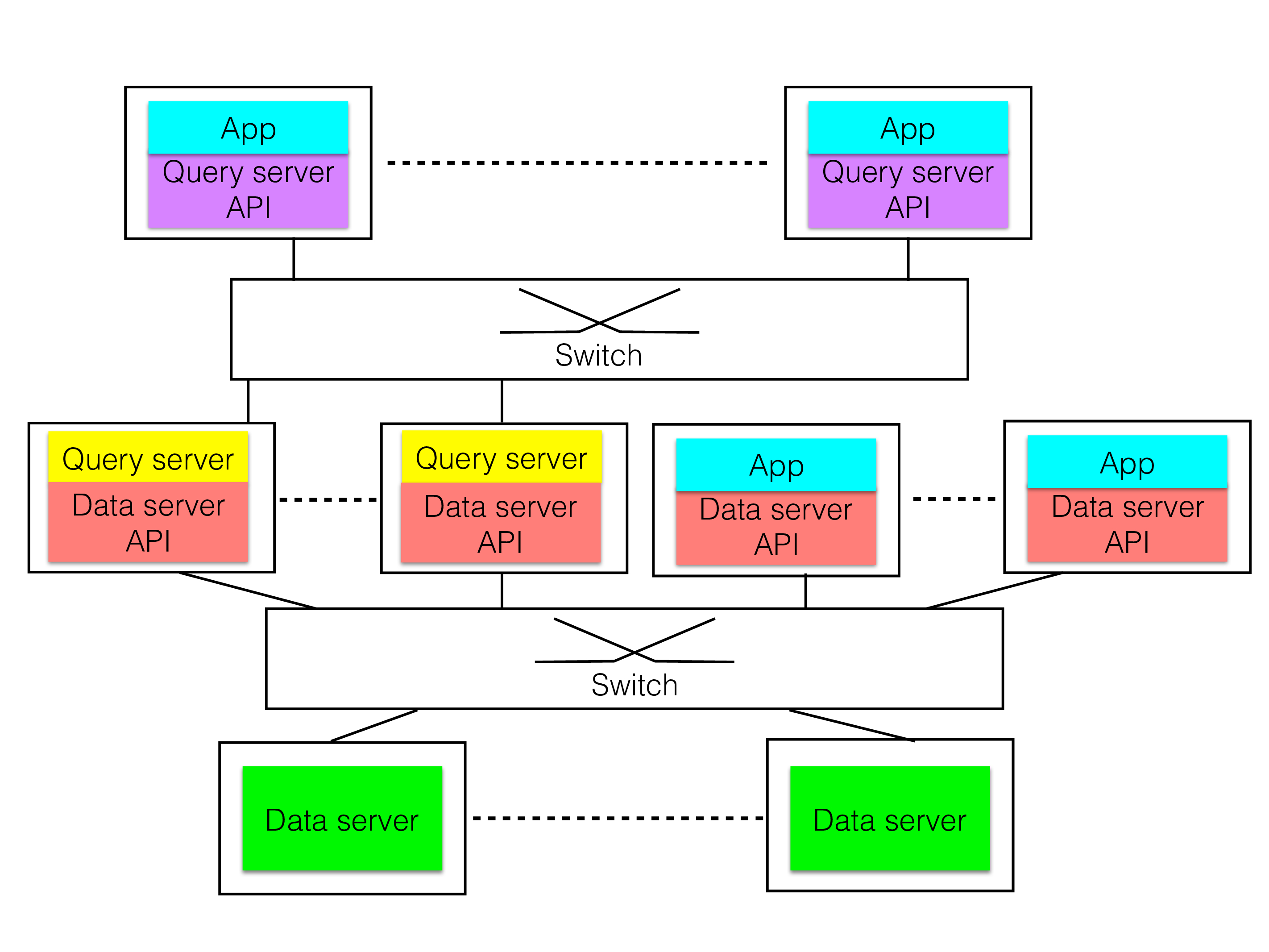
Most traditional DBMSs used in high-availability setups use a shared-disk approach as shown by the figure above. Shared-disk architecture means that the disks are shared by all nodes in the cluster. In reality, the shared disks are a set of storage servers, implemented either by software or a combination of hardware and software. Modern shared-disk DBMSs mostly rely on pure software solutions for the storage server part.

Shared-disk has advantages for query throughput in that all data is accessible from each server. This means that it reads data from the storage server to perform its queries. This approach has limited scalability but each server can be huge. In most cases, the unit transported between Storage Server and Data Server is pages of some standard size such as 8 kByte.

It is very hard to get fast failover cases in a shared-disk architecture since it is necessary to replay the global REDO log as part of failover handling. Only after this replay can pages that was owned by a failed node be read or written again.

This is the reason why all telecom databases use the shared-nothing approach instead as shown in the figure below. With shared-nothing the surviving node can instantly take over, the only delay in taking over is the time it takes to discover that the node has failed. The time it takes to discover this is mostly dependent on the operating system and a shared-nothing database can handle discovery and take over in sub-second time if the OS supports it.

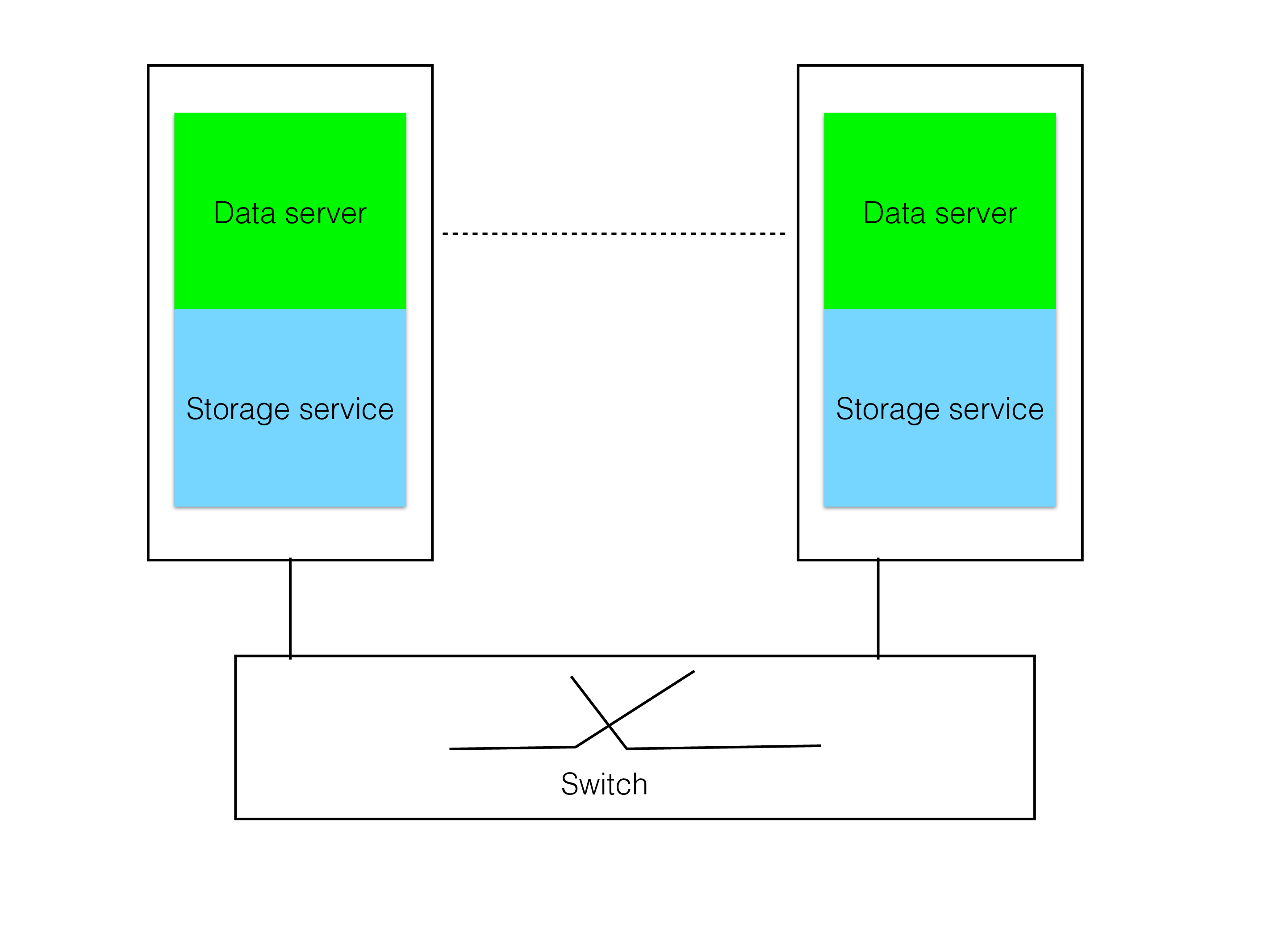
An interesting note is that shared-disk implementations depend on a high-availability file system that is connected to all nodes. The normal implementation of such a high-availability storage system is to use a shared-nothing approach. Interestingly RonDB could be used to implement such a high-availability storage system. It is an intriguing fact that you can build a highly available shared-disk DBMS on top of a storage subsystem that is implemented on top of RonDB.

RonDB and the CAP theorem

The CAP theorem says that one has to focus on a maximum of two of the three properties Consistency, Availability and Partitioning where partitioning refers to network partitioning. RonDB focuses on consistency and availability. If the cluster becomes partitioned we don’t allow both partitions to continue, this would create consistency problems. We try to achieve the maximum availability without sacrificing consistency.

We go a long way to ensure that we will survive as many partitioning scenarios as possible without violating consistency. We will describe this in a later chapter on handling crashes in RonDB.

However, there is more to the CAP theorem and RonDB. We support replicating from one cluster to another cluster in another part of the world. This replication is asynchronous. For replication between clusters we sacrifice consistency to improve availability in the presence of Partitioning (network partitioning). The figure below shows an architecture for replication between two clusters. As can be seen here it is possible to have two replication channels. Global replication is implemented using standard MySQL Replication where the replication happens in steps of a group of transactions (epochs).

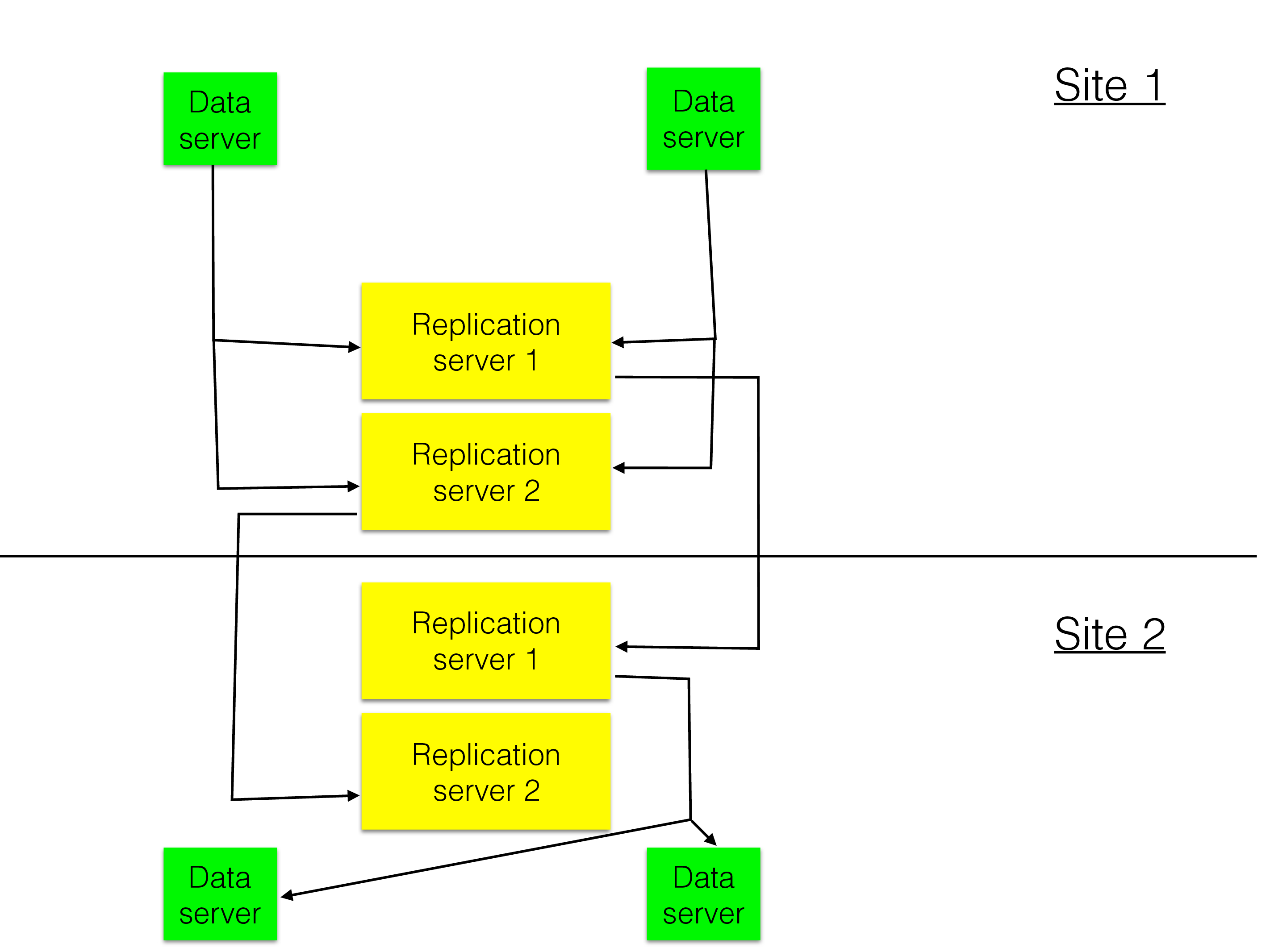
If the network is partitioned between the two clusters (or more than two clusters) then each cluster will continue to operate. How failures are handled here is manually handled (implemented as a set of automated scripts that might have some manual interaction points).

RonDB gives the possibility to focus on consistency in each local cluster but still providing the extra level of availability by handling partitioned networks and disasters hitting a complete region of the world. Global replication is implemented and used by many users in critical applications.

The replication between clusters can support writing in all clusters with conflict resolution. More on this in the chapter on RonDB Replication.

OLTP, OLAP and relational models

There are many DBMSs implemented in this world. They all strive to do similar things. They take data and place it in some data structure for efficient access. DBMSs can be divided into OLTP (Online Transaction Processing) and OLAP (Online Analytical Processing). There are databases focused on special data sets such as hierarchical data referred to as graph databases, other types are specialized DBMSs for geographical data (GIS). There is a set of DBMSs focused on time-series data.

The most commonly used DBMSs are based on the relational model. Lately, we have seen the development of numerous Big Data solutions. These data solutions focus on massive data sets that require scaling into thousands of computers and more. RonDB will scale to hundreds of computers but will do so while maintaining consistency inside the cluster. It will provide predictable response times even in large clusters.

RonDB is a DBMS focused on OLTP, one of the most unique points of RonDB is that 1 transaction with 10 operations takes a similar time to 10 transactions with 1 operation each. An OLTP DBMS always focuses on row-based storage and so does RonDB. An OLAP DBMS will often focus on columnar data storage since it makes scanning data in modern processors much faster. At the same time, the columnar storage increases the overhead in changing the data. RonDB uses row storage.

Data storage requirements

In the past, almost all DBMSs focused on storing data on disk with a page cache. In the 1990s the size of main memory grew to a point where it was sometimes interesting to use data which always resides in memory. Nowadays most major DBMS have a main memory options, many of those are used for efficient analytics, but some also use it for higher transaction throughput and best possible response time.

RonDB chose to store data in main memory mainly to provide predictable response time. At the same time, we have developed an option for tables to store some columns on disk with a page cache. This can be used to provide a much larger data set stored in RonDB using SSD storage. Disk data is primarily intended for use with SSDs since most current RonDB applications have stringent requirements on response time.

RonDB and Big Data

RonDB was designed long before Big Data solutions came around, but the design of RonDB fits well into the Big Data world. It has automatic sharding of the data, queries can get data from all shards in the cluster. RonDB is easy to work with since it uses transactions to change data which means that the application won’t have to consider how to solve data inconsistencies.

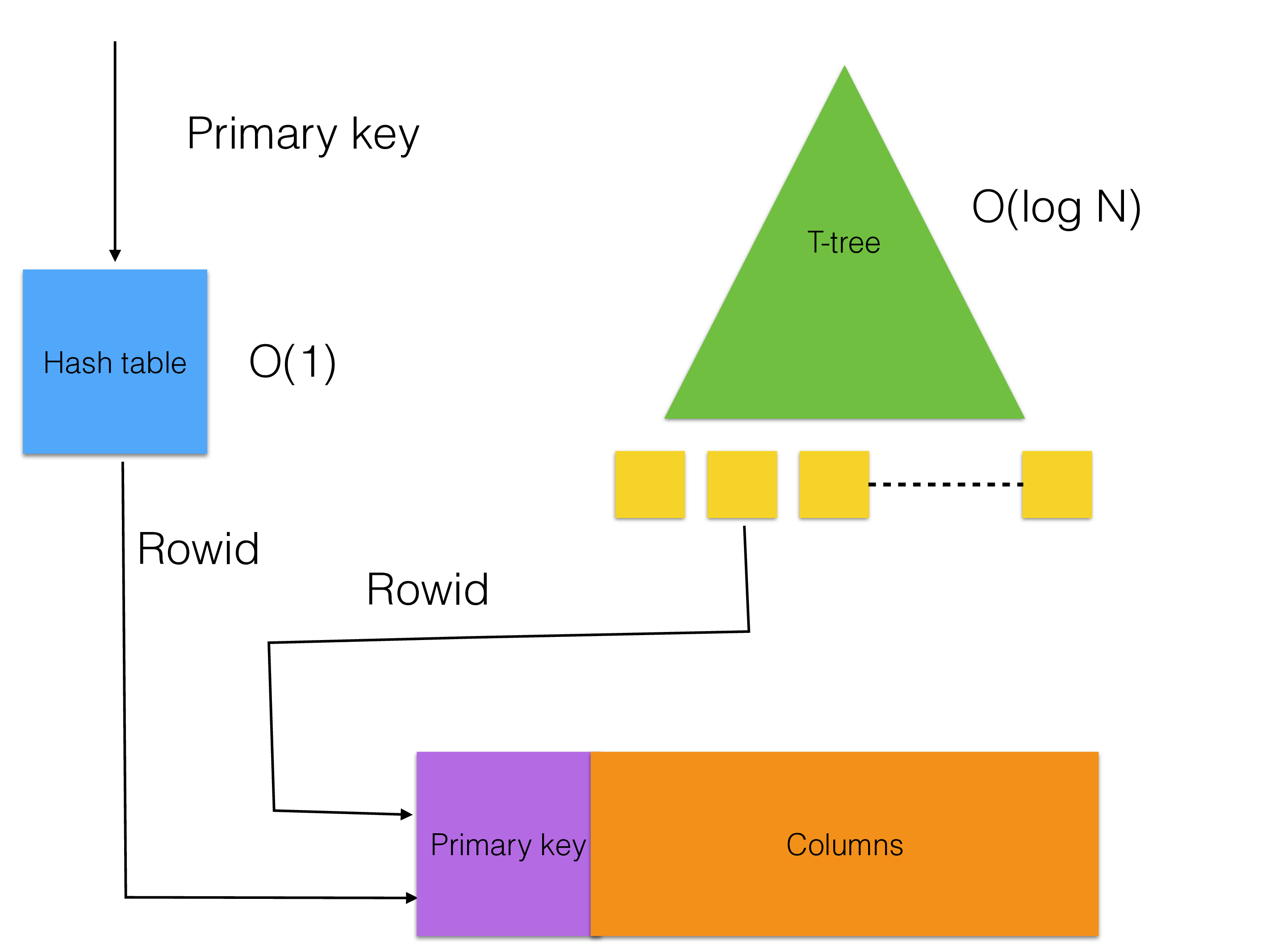
The data structures in RonDB are designed for main memory. The hash index is designed to avoid CPU cache misses and so is the access to the row storage. The ordered index uses a T-tree data structure specifically designed for main memory. The page cache uses a modern caching algorithm that takes into account both data in the page cache as well as data that has since long been evoked from the page cache when making decisions of the heat level of a page.

Thus the basic data structure components in RonDB are all of top-notch quality which gives us the ability to deliver benchmarks with 200 million reads per second and beyond.

Unique selling point of RonDB

The most important unique selling points for RonDB comes from our ability to failover instantly, to be able to add indexes, drop indexes, add columns, add tables, drop tables, add node groups and reorganize data to use those new node groups, change software in one node at a time or multiple at a time, add tablespaces, add files to tablespaces. All of these changes and more can all be done while the DBMS is up and running and all data can still be both updated and read, including the tables that are currently changed. All of this can happen even with nodes in the cluster leaving and joining. The most unique feature of RonDB is AlwaysOn. It is designed to never go down, only bugs in the software or very complex changes can bring down the system and even that can be handled most of the time by using MySQL replication to a backup cluster.

There are many thousands of NDB clusters up and running that have met tough requirements on availability. Important to remember here is that to reach such high availability requires a skilled operational team and processes to handle all types of problems that can occur and of course 24x7 support.