Relation Model

Before introducing the model of how RonDB works we will introduce the terminology, this chapter introduces the relational model in a distributed system together with some concepts related to this that are used in RonDB. The following chapter will introduce the model for distributed transactions and the terminology chapter will introduce the model we use for processors, computers and operating systems.

Basic concepts

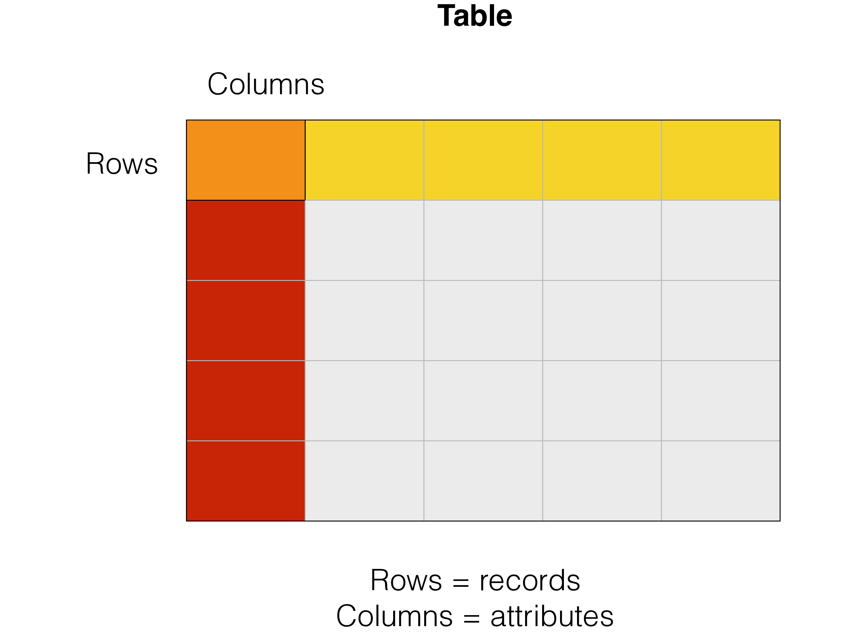
A database is used to store information, this information is represented as values that can be of many different data types. More or less every conceivable database solution organises its data into records. A record can consist of one or more attributes. Synonyms for attributes are columns and fields. A synonym for record is row.

The physical storage in a database is usually organised in records for Online Transaction Processing (OLTP) DBMSs and often organised column-wise for Online Analytical Processing (OLAP) DBMSs. In RonDB the physical storage is organised in records although we separate the storage into fixed size columns, variable sized columns and disk columns.

A column can only contain a single value according to the relational model. Most relational DBMSs does however allow for various complex objects stored in Binary Large OBjects (BLOBs).

In order to organise data it is common to employ some sort of schema to describe the data. It is possible to avoid the schema, in this case each row will have to contain the schema describing the row.

The relational model employs a strict schema which only allows storage of a single value per attribute and that each table has a fixed set of attributes. Representation of multi-valued attributes in the relational model is done by a separate table that can later be joined with the base table to retrieve the multi-valued attributes.

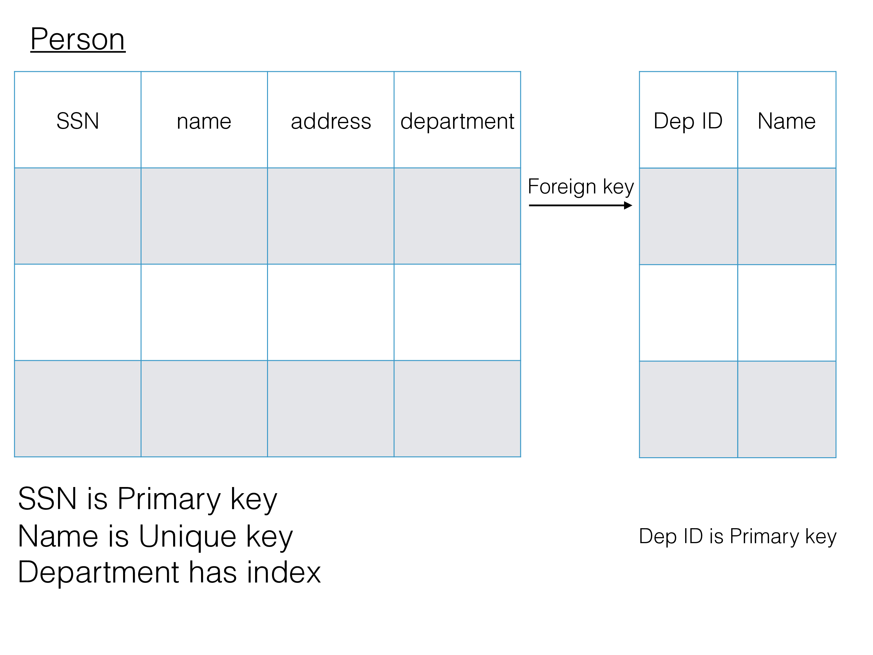
Another key concept in the relational model is primary key, this is a unique reference to a row in the table. If several unique identifiers exist in a table these are unique keys, only one primary key can exist in a table. Both primary key and unique keys are implemented using indexes that ensure uniqueness. In addition many non-unique indexes can be defined on a table.

Foreign keys defines relational constraints between tables in the schema. A foreign key above in the table person (child table) refers to a row in the department table (the parent table). The child table has a unique reference to the row in the parent table. Normally the columns defining the foreign key relation has an index defined on them (it is a requirement in RonDB). The above figure shows an example of this.

There are other models where one describes the schema in each row. The popular format JSON follows this model.

The relational model was introduced in the 1970s by IBM. It is a simple model that provides nice mathematical properties that makes it easy to reason about the relational model and that makes it easy to develop complex queries against data and still be able to deduce how to compute the results of those queries.

One benefit of the relational model is that it is easy to reason about queries in this model. For example a select of a subset of the rows in a table and a projection only reading a number of columns delivers a query result which in itself is a table. A table can be joined with another table (or joined with a select-project of another table). The result of a join is again something that is a table. The result of a join can be joined with yet another table. In this manner a query can be arbitrarily complex. Sometimes this is called select-project-join. We have pushed some of this functionality down into the data server part and call the module that handles this DBSPJ where SPJ comes from Select-Project-Join. There are many types of joins, equality joins, semi-joins, cross product and so forth.

During the early phases of developing an application it is not crystal clear how the data model will look like. Thus the model constantly changes. As development progresses the model tends to be more and more fixed and changes are often expensive. This is true independent of how schemas are stored. This is just how development for any application happens.

If all records have their own schema we can end up with quite a messy data model at the end. In coding one talks about spaghetti code and similar here it is easy to end up with a spaghetti data model if there is no control of the development of the schema.

With RonDB we want to make it easy to change the schema dynamically in the early phases of development and in later phases of the development. At the same time we want to get the benefits of the relational model and its strength in handling complex queries.

We have implemented a data structure for records where it is easy to add and drop columns. The record representation is fixed per table, but it is easy to add and drop attributes on a table. The table can continue to be updated while these attributes are added (online drop column is not yet supported).

Thus in RonDB (as in MySQL) you define a table to consist of a set of attributes with a table name.

As most modern implementations of relational DBMSs RonDB have added support for BLOBs (Binary Large OBjects) of various sizes and types such as GIS types and JSON objects (these are BLOBs that contain a self-described document, containing its own schema per document).

Distributed Relational Model

RonDB is a distributed database as well. Thus the table has to be partitioned and replicated in some fashion as well. We selected horisontal partitioning in RonDB. Thus each row is mapped to one partition of the table. Each partition contains a subset of the rows, but it contains all attributes of the table for the rows it stores.

We use the term partition for the table partitions, but internally and in some documentation we have used the term fragment. We tend to nowadays use the term partition for the partitioning as seen by the user and to use the term fragment internally. One reason for this is that with fully replicated tables one partition is implemented as multiple fragments that are copies of each other.

Replicated Relational Model

RonDB employs replication to ensure that data remains available in the presence of failures. We need a model to map the replicas to nodes. In RonDB we have selected a mapping model that maximises the amount of node crashes we can survive. One could have employed a model where we spread the replicas in such a way that we optimise for fastest possible restart times. But the fastest restart time model can only handle one node crash which isn’t good enough for high availability in a large cluster.

The model we have selected means that we group the nodes into node groups. One fragment is always fully replicated within one node group and there are no fragment replicas in any other node group. Thus if we have 2 replicas we can survive one node crash in each node group and with more replicas we can survive even more node crashes.

Node groups divides data in the same manner as done for sharding. Therefore one of the features of RonDB is that it handles auto-sharding.

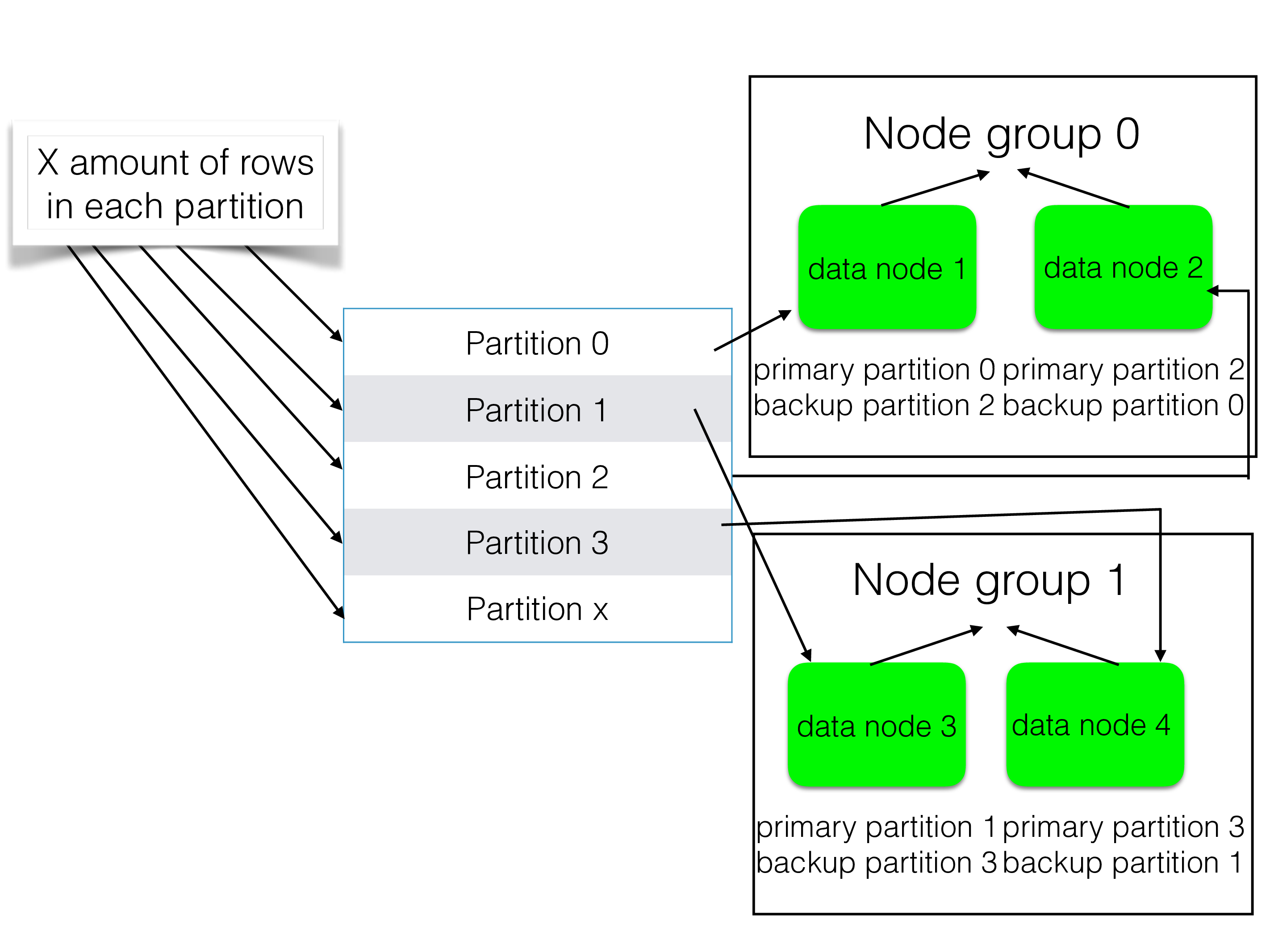
As the figure shows the row decides which partition the row goes into. The partition decides the node group the fragment replicas are stored in. Each partition has one primary fragment replica and one or more backup fragment replicas.

There can be a maximum of 144 data nodes and with 2 replicas this means a maximum of 72 node groups.

RonDB have its own heartbeat handling, when a node dies it will stop sending heartbeats, the neighbour nodes will discover the node failure and at failure the surviving nodes that can communicate with each other will work together in definining a new cluster setup with the remaining nodes.

We have to handle the case where network partitioning can occur. The simplest case is two data nodes and the network between those nodes is broken. In this case both nodes will attempt to form a new cluster setup. If both nodes are allowed to survive we will have two databases which is something we want to avoid.

To handle this situation we use another node in the cluster that doesn’t own any data as arbitrator. This node will decide which set of nodes that should survive. The arbitrator is only contacted if a network partitioning is possible, the first one to contact it will win.

Hashmaps

Tables in RonDB use a concept called hashmaps. Hashmaps were introduced to make it easy to reorganize tables when new node groups are created. The algorithm we use to find the record based on a key is called distributed linear hashing and was named $LH^3$ in my Ph.D thesis. The linear hashing algorithm makes it possible to dynamically grow and shrink the hash table. There is one drawback for table reorganisation, the drawback is that when we have e.g. 6 partitions the first 4 partitions will contain 75% of the data (thus 18.75% per partition) and the last 2 partitions will contain 25% of the data and thus 12.5% per partition. Thus we won’t have a balanced data fragmentation as is desirable.

The solution is hashmaps. We will hash into one of the 3840 buckets in the hashmap. Next we will map the bucket in the hashmap into the partition it should be stored in. When reorganising a table we simply change the mapping from hashmap bucket to partition. The fragmentation will thus be a lot more balanced than the traditional linear hash algorithm.

With RonDB we support online add of columns, online add/drop of tables, online reorganization of tables to handle new nodegroups introduced or to handle change of table distribution.

By default a table is divided into 3840 hashmap buckets. This means that if we have 8 partitions in a table each partition will house 480 hashmap buckets. If we add a new nodegroup such that we double the number of partitions, each partition will have 240 hashmap buckets instead. The original partitions will move away 240 out of the 480 hashmap buckets to the new partitions, the rest will stay. This is one more idea of hashmaps, to make sure that we can always reorganize data and that as much data as possible don’t have to move at all.

The number 3840 is selected to make table distributions balanced in as many cases as possible without creating a hashmap which is too big. If we find the prime numbers in 3840 we see that 3840 = 2 * 2 * 2 * 2 * 2 * 2 * 2 * 2 * 3 * 5

Thus we can handle completely balanced distributions as long as the number of partitions can be made up a product of the prime numbers in 3840. E.g. if we have 14 nodes in the cluster we will not get perfect balance since 14 is 2 times 7 and 7 is not a prime number in 3840. The number of partitions for a default table is 2 times the number of nodes.

This means that we won’t necessarily have balance on the use the data owning threads (ldm threads). We have solved this by introducing query threads that can assist a set of ldm threads with reads. Combining this with some advanced scheduling of local queries inside a data node ensures that the CPUs in the data nodes gets a balanced load.

Read backup replica tables

In earlier versions of RonDB the focus was to provide a write scalable architecture. We have added an option that makes it possible to have tables scale better for reading. This is now the default behaviour. This is an option when creating the table (or one can set the option in the MySQL Server if all tables should use this option). With this option READ_BACKUP=1 the reads can go to any fragment replica where the row is stored. There is a tradeoff with this in that write transactions will be slightly delayed to ensure that the reads can see the result of their own changes in previous transactions. We will explain more about the need for this special type of flags when we introduce the distributed transaction protocol that RonDB uses.

Fully replicated tables

RonDB also supports a type of table which is called fully replicated tables, these tables can always read any replica for read committed queries. Normal tables in RonDB have different data in each node group. For a fully replicated table we have the same data in each node group. There is still be a number of partitions, but each node group has the same set of fragments and they are replicas of each other. When a transaction changes a row in a fully replicated table it will change all replicas. It does this by using an internal trigger, the main fragment is first updated, a trigger ensures that all copy fragments are updated as well. All those changes are part of the same transaction, thus the update is atomic.

Fully replicated tables makes it possible to build simple read scalability into your applications. A natural architecture is to have one MySQL Server and one RonDB data node per machine that can communicate without using networking equipment. In this manner we can have up to 144 machines with the same data delivering many millions of SQL queries against the same data. Any changes are done to all replicas synchronously, no need to worry about replication lags and things like that.

Fully replicated tables can be reorganised, it is possible to start with a 2-node cluster and grow in increments of 2 until we reach 144 nodes. Similarly one can start with 3 replicas and grow in increments of 3 until we reach 144 nodes and similarly with 4 replicas. Reorganising a fully replicated table doesn’t change the number of partitions, it only creates a number of new copy fragments of the partitions in the new node group(s).